Making zooplankton swim with random walks

To get started we need a couple of libraries for plotting. For the main plotting we will use ggplot2, gganimate is useful to turn the plots into gifs, and ggimage is going to let us add a daphnia to the plot.

library(ggplot2)
library(gganimate)
library(ggimage)

What is a random walk?

In one dimension our random walker can move forward or backward (or up/down). The distance they move is drawn from some distribution, here we are using a standard normal distribution. The standard normal is symmetrical around 0, which means that there is an equal probability of moving forward or backwards, and there is a higher probability of moving short distances.

To simulate a simple random walk along the x axis for 100 time steps, we can use the cumsum function with rnorm. The rnorm allows us to sample random values from a normal distribution with a mean of 0 and a standard deviation of 1 (aka the standard normal). The cumsum function then computes the cumulative sum of these values. If, for example our first three values from rnorm were 0.89, -0.395, and 2.11 then the cumulative sum would be 0.89, followed by 0.495 (0.89 - 0.395), and then 2.605 (0.495 + 2.11). We will also set all y values equal to 0, because we want the random walk to only be along the x axis.

df <- data.frame(time = 1:100, x = cumsum(rnorm(100, 0, 1)), y = 0)

The data frame now contains values for 100 time steps, with a new x value each step. We can visualize this with an animation using the gganimate package. Set x = x, and y = y, and use a point to represent our random walker. Adding transition_time tells R that we want the gif to step forward in time according to the time column.

ggplot(df, aes(x = x, y = y)) + geom_point(size = 4) + 
  theme_bw(base_size = 14) + 
  transition_time(time)

For a bit of added fun, we can replace geom_point with geom_image from the ggimage package. Adding a link to the desired image, in this case to Daphnia (a ubiquitous zooplankton), as an additional column in the data frame lets us use the image in place of the point. Now we have a Daphnia swimming along the x-axis.

df <- data.frame(time = 1:100, loc = cumsum(rnorm(100, 0, 1)), y = 0, img = "http://phylopic.org/assets/images/submissions/ef7610ee-e767-46d5-a2e5-9e474ed50c10.64.png")

ggplot(df, aes(x = loc, y = y)) +   
  geom_image(aes(image = img)) + 
  theme_bw() + 
  transition_time(time)

Ok that’s great, but how often do we think in 1 dimension? How can we make this better by also allowing our Daphnia to swim vertically. In this case, we can treat the y column of the data frame in the same way we set x, using the same cumsum and rnorm functions. At this point I should note that there is no reason you have to use a standard normal, and you could replace rnorm with any sampling distribution (and there are a lot available in R). Though if you choose a distribution with only positive values (looking at you rlnorm, rpois, and rgamma among others) then the random walker can only move forward. You can get around this by multiplying sampled values by sample(c(-1,1), 1), which randomly samples either 1 or -1 with equal probability and thereby changing a positive distribution to one symmetrical about 0.

df <- data.frame(time = 1:100, x = cumsum(rnorm(100, 0, 1)), y = cumsum(rnorm(100, 0, 1)), img = "http://phylopic.org/assets/images/submissions/ef7610ee-e767-46d5-a2e5-9e474ed50c10.64.png")

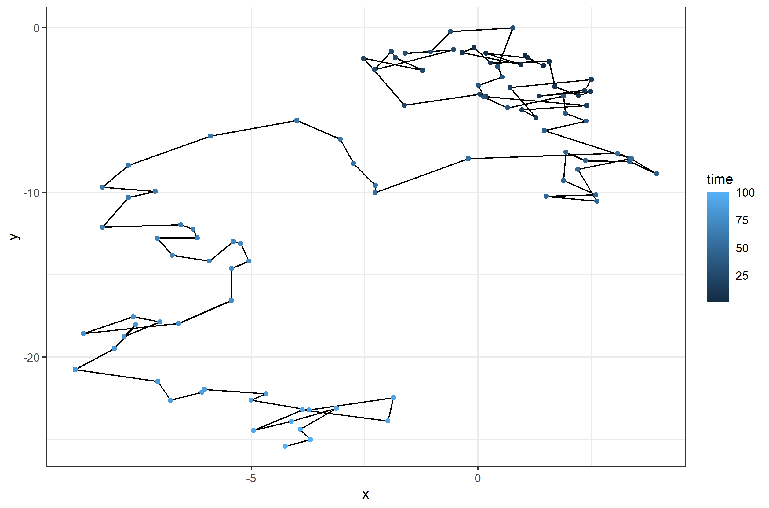
First, lets take a look at the path taken by the random walker in 2 dimensions. In the plot below you can see the different steps taken along the walk, with the path becoming lighter as we near the end of the time series.

ggplot(df, aes(x = x, y = y)) + geom_path() +  
  geom_point(aes(color = time)) + 
  theme_bw()

Now we can watch it all unfold as the Daphnia swims around.

ggplot(df, aes(x = x, y = y)) +
  geom_image(aes(image = img)) + 
  theme_bw() + 
  transition_time(time)  

Look at that little guy bounce around… Now that we have the basics down, we can get a little fancier.

First, I downloaded two images. One was the Daphnia image (you can get here) I used before so that I have it locally, and the other is a copepod, which is a different zooplankton (you can get here).

daphnia_img <- "PhyloPic.ef7610ee.Anomopoda_Cladocera_Daphnia_Daphniidae.png"
cop_img <- "PhyloPic.c5dbd85a.Joanna-Wolfe.Calanoida_Copepoda_Epacteriscidae_Erebonectes_Gymnoplea_Neocopepoda.png"

Now, we are going to have 5 individuals, 3 Daphnia and 2 copepods, so we define a data frame for each individual. Then, we combine them all together into one long data frame with do.call and rbind. That is why we include a column called sp as an identifier for each unique individual for plotting (though we don’t need it for what we are doing now).

df1 <- data.frame(time = 1:100, x = cumsum(rnorm(100, 0, 1)), y = cumsum(rnorm(100, 0, 1)),
                  img = daphnia_img, sp = "A")
df2 <- data.frame(time = 1:100, x = cumsum(rnorm(100, 0, 1)), y = cumsum(rnorm(100, 0, 1)),
                  img = daphnia_img, sp = "B")
df3 <- data.frame(time = 1:100, x = cumsum(rnorm(100, 0, 1)), y = cumsum(rnorm(100, 0, 1)),
                  img = daphnia_img, sp = "C")
df4 <- data.frame(time = 1:100, x = cumsum(rnorm(100, 0, 1)), y = cumsum(rnorm(100, 0, 1)),
                  img = cop_img, sp = "D")
df5 <- data.frame(time = 1:100, x = cumsum(rnorm(100, 0, 1)), y = cumsum(rnorm(100, 0, 1)),
                  img = cop_img, sp = "E")

allpaths <- do.call(rbind, list(df1, df2, df3, df4, df5))

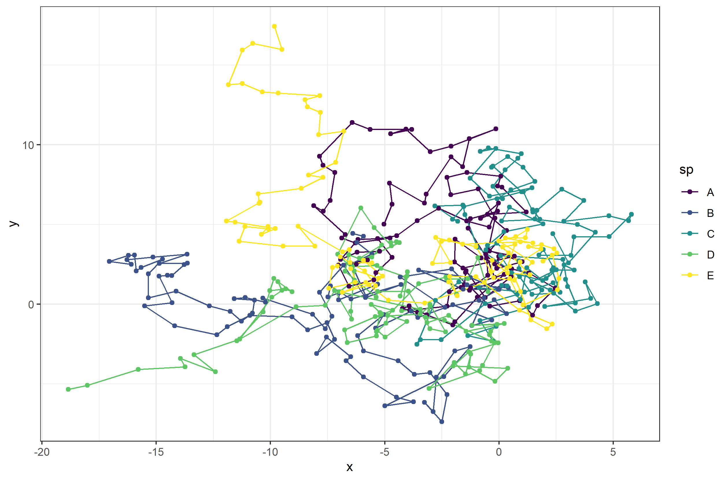
Let’s take a look at the path our 5 random walkers will take.

ggplot(allpaths, aes(x = x, y = y, color = sp)) + 
  geom_path() +  
  geom_point() + 
  scale_color_viridis_d() + 
  theme_bw()

Now let’s animate it, and this time, we can add in some extras. First, we add a title to tell us what time step we currently are at. Next, to give us more control over the animation, we can save the ggplot object and then animate it witht he animate function. Using the animate function lets us set the number of frames and more for the gif.

anim_allind <- ggplot(allpaths, aes(x = x, y = y)) + geom_point() +  
  geom_image(aes(image = img)) + 
  labs(title = "Timestep: {round(frame_time,0)}") + 
  theme_minimal() + 
  transition_time(time)
animate(anim_allind, nframes = 200)

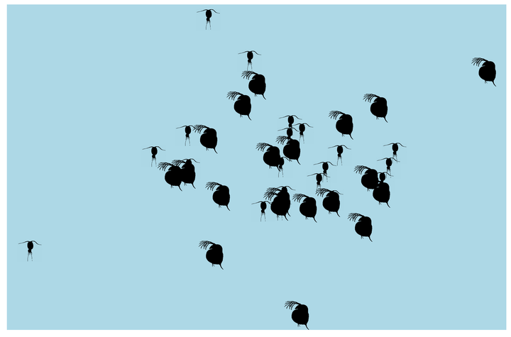
What if we made it look a bit more like a lake or pond that we would find these plankton in? Get rid of the grid elements, axis text, ticks, and lines. Add a few more frames for smoother transitions, and make the background blue.

anim_pond <- ggplot(allpaths, aes(x = x, y = y)) + geom_point() +  
  geom_image(aes(image = img)) + 
  theme(panel.background = element_rect(fill = "lightblue"), 
        panel.grid = element_blank(), 
        axis.title = element_blank(), axis.line = element_blank(), 
        axis.text = element_blank(), axis.ticks = element_blank()) + 
  transition_time(time) 
animate(anim_pond, nframes = 400)

If we want a whole bunch of individuals to be randomly walking around our little pond, instead of defining each data frame individually, we can use lapply to create a list of data frames automatically. Here we define two lists, one for Daphnia and one for copepods, each with 20 individuals. I’ve also changed the code a bit, so that the initial starting point is drawn from a wider distribution, so they start off a bit more spread out. I also changed the standard deviation of the normal distribution for each step to be randomly drawn from 1 to 5. That way each individual is going to move different distances (though in this case the standard deviation remains the same for any given individual throughout the simulation).

dlist <- lapply(1:20, function(x){
  data.frame(time = 1:101, x = cumsum(c(rnorm(1, 0, 10),rnorm(100, 0, sample(1:5, 1)))),
             y = cumsum(c(rnorm(1, 0, 10),rnorm(100, 0, sample(1:5, 1)))),
             img = daphnia_img, sp = "A")
})

clist <- lapply(1:20, function(x){
  data.frame(time = 1:101, x = cumsum(c(rnorm(1, 0, 10),rnorm(100, 0, sample(1:5, 1)))), 
             y = cumsum(c(rnorm(1, 0, 10),rnorm(100, 0, sample(1:5, 1)))),
             img = cop_img, sp = "B")
}) 

npaths <- do.call(rbind, list(do.call(rbind, dlist), do.call(rbind, clist)))

npath_pond <- ggplot(npaths, aes(x = x, y = y)) + geom_point() +  
  geom_image(aes(image = img)) + 
  theme(panel.background = element_rect(fill = "lightblue"), 
        panel.grid = element_blank(), legend.position = "none",
        axis.title = element_blank(), axis.line = element_blank(), 
        axis.text = element_blank(), axis.ticks = element_blank()) + 
  transition_time(time) 
animate(npath_pond, nframes = 400)

From here it would be a good exercise to turn this code into a function, where you could define the number of time steps and the number of individuals, and create the data frame for plotting without having to rewrite a bunch of code each time.